What is LiDAR? Working Principles, Applications, and Choosing the Right Sensor for Robotics
Executive Hook: The Paradigm Shift in Autonomous Navigation
Look, if you are building warehouse robots, heavy duty AGVs, or commercial unmanned aerial vehicles (UAVs) today, spatial awareness is no longer some optional luxury feature. It is a hard baseline operational requirement. In the shop, we have all watched traditional sensing technologies like ultrasonic sensors and basic optical cameras hit a physical wall. They consistently struggle to deliver the kind of clean, high-fidelity, real-time 3D spatial data you need for high-velocity obstacle avoidance, SLAM (Simultaneous Localization and Mapping), and tight cargo handling. That is where LiDAR (Light Detection and Range) comes in to save the day. By using active, time-of-flight laser emission, modern LiDAR modules reconstruct surrounding environments with millimeter-to-centimeter precision, working beautifully whether you are inside a dark distribution center or outside in an open yard blasted by direct noon sunlight.
Here is the deal for engineering teams, system integrators, and robotics developers: choosing the right LiDAR architecture means balancing tough trade-offs. You are looking at weight budgets, payload capacities, processing throughput limits, environmental survivability, and communication physical layers. This guide tears down the underlying physics of LiDAR technology, categorizes modern architectural variations, clarifies critical performance metrics, and introduces industrial-grade solid-state dToF (Direct Time-of-Flight) sensor design. Our goal is simple: skip the marketing fluff and give you the mechanical and optical intuition to rapidly pick and integrate the most efficient depth sensor for your autonomous mobile robot (AMR) or unmanned platform.
Table of Contents
- 👉 Module 1: The Physics of Light Detection and Ranging (LiDAR)
- 👉 Module 2: Component Architecture of Industrial LiDAR Sensors
- 👉 Module 3: Taxonomy of LiDAR Designs: Mechanical vs. Solid-State
- 👉 Module 4: Critical Performance Evaluation Metrics for Robotics Integration
- 👉 Module 5: Technical Specification Blueprint: Solid State LiDAR HM-LD1
- 👉 Module 6: Software Integration & Embedded Developers SDK Ecosystem
- 👉 Module 7: Developer Knowledge Hub (FAQ)
Module 1: The Physics of Light Detection and Ranging (LiDAR)
At its mathematical and physical core, LiDAR operates on the clean principle of optical Time-of-Flight (ToF). By emitting a highly collimated stream of electromagnetic radiation outer-bound of the visible spectrum and measuring exactly how long it takes for that signal to hit a reflective target and bounce back to a co-located optical sensor, the system accurately computes the absolute physical distance along the ray’s vector. We are talking about converting time directly into highly accurate spatial positioning.
The structural calculation of distance (represented as d) is derived directly from the invariant speed of light in a given medium. This calculation relies on the formula:
d = (c · Δt) / (2 · n)
Where c represents the speed of light in a vacuum (approximately 3 × 10⁸ meters per second), n corresponds to the refractive index of the medium (with air measuring approximately 1.00027 under standard atmospheric temperature and pressure), and Δt represents the total elapsed time-of-flight. The division by two accounts for the round-trip distance, as the light pulse must travel out to the target and return back to the active photo-detector. To resolve millimeter-level steps in physical spatial measurements, the timing circuitry of the detector must resolve picosecond-scale (10-12 seconds) intervals. This level of processing precision is exactly what separates industrial-grade active sensing components from cheap consumer toys.
Direct Time-of-Flight (dToF) vs. Indirect Time-of-Flight (iToF)
Modern depth-sensing designs are fundamentally split into two measurement methodologies: Direct Time-of-Flight (dToF) and Indirect Time-of-Flight (iToF). Each architecture has distinct performance trade-offs under varying ambient light conditions and physical ranges. Let’s look at how they stack up on the test bench:
- ✅ Direct ToF (dToF): In a dToF architecture, the sensor fires a discrete, sub-nanosecond optical pulse. Upon emission, an ultra-fast internal system clock—typically an integrated Time-to-Digital Converter (TDC)—begins counting. When the reflected photons impact the pixel surface of the photo-detector, the TDC stops the clock, capturing the actual elapsed time directly. dToF is exceptionally resilient to multipath interference (where light bounces off multiple surfaces before returning) because it isolates single pulse peaks. It scales efficiently to long-distance designs without requiring exponentially increased optical output power. This makes it excellent for outdoor applications where solar ambient noise is high, as the instantaneous power of the laser pulse easily towers over steady-state background lux. Built on SPAD (Single-Photon Avalanche Diode) matrices, this technology is utilized in state-of-the-art designs such as Sony’s advanced SPAD dToF sensor families.
- ⚙️ Indirect ToF (iToF): Spatial mapping via iToF does not trace individual pulses directly. Instead, the emitter sends a continuously modulated continuous wave (CW)—typically a sinusoidal or square-wave signal. The receiver measures the phase shift (Δφ) between the transmitted and received waveforms across multiple modulation frequencies to deduce depth. While offering spatial resolutions that match the megapixel layouts of standard CMOS imagers (making it simple to manufacture and inexpensive for short-range deployments), iToF has physical limitations. It exhibits high susceptibility to multipath errors (or “phase wrapping”), which distorts corner measurements, and suffers from heavy power consumption since the emitter remains in a near-continuous state of transmission. Furthermore, ambient sunlight easily saturates the detector wells, rendering it less effective in outdoor environments.
Single-Photon Avalanche Diode (SPAD) Receiver Mechanics
To achieve highly accurate long-range measurements under restrictive eye-safety regulations (Class 1 laser limits), modern LiDAR sensors rely on Single-Photon Avalanche Diode (SPAD) detector arrays. A SPAD is a semiconductor p-n junction biased above its breakdown voltage (known as the Geiger mode). In this metastable state, a single incoming photon striking the depletion region can trigger a cascade of secondary impact-ionization events, causing a massive avalanche current (105 to 106 electron-hole pairs generated per photo-generated charge carrier). This avalanche is rapidly extinguished via active or passive quenching circuitry to reset the diode for the next photon arrival event.
Through statistical processing of thousands of these avalanche triggers in a Time-Correlated Single-Photon Counting (TCSPC) register, SPAD sensors reconstruct an accurate histogram of photon return times. This mechanism enables SPAD-based dToF LiDARs to detect fragile optical echoes returning from low-reflectivity objects (such as dark plastics, matte black painted steel, or wet asphalt), even when masked by high solar background illumination. In short, it lets you pull clean signals out of incredible amounts of ambient noise.
Module 2: Component Architecture of Industrial LiDAR Sensors
From an integration standpoint, an industrial-grade LiDAR is a complex optoelectronic machine. In the field, you cannot treat it like a simple black box. You have to understand how the emitter and receiver pathways interact to survive harsh operational environments.
1. Laser Emitters & Wavelength Options
The choice of wavelength limits target reflectivity, system eye safety boundaries, production manufacturing costs, and optical sensitivity.
- ⚙️ 905 nanometers (GaAs Near-Infrared – NIR): Silicon photodetectors remain highly sensitive at this wavelength, meaning 905nm LiDAR systems can utilize integrated, high-volume silicon CMOS receivers. This vastly lowers component prices. The primary challenge is eye safety: because 905nm light readily penetrates the human eye and focuses onto the retina, strict international standards (IEC 60825-1) restrict the maximum allowable pulse energy. This caps the physical range of 905nm sensors unless advanced, ultra-sensitive SPAD matrices are utilized to register ultra-weak returning signals.
- ⚙️ 1550 nanometers (InGaAs Short-Wave Infrared – SWIR): Light at 1550nm is strongly absorbed by the cornea and lens of the human eye before reaching the retina, allowing for laser power emissions roughly 100 times higher than 905nm designs while remaining eye-safe. This yields incredible outdoor detection ranges exceeding 200 meters. However, silicon-based sensors are transparent to 1550nm light. Custom Indium Gallium Arsenide (InGaAs) detectors are required, raising manufacturing costs and making them cost-prohibitive for compact indoor mobile robot fleets.
- ⚙️ Emitter Technology Types: Modern solid-state LiDARs are moving away from legacy Edge-Emitting Lasers (EELs) toward Vertical-Cavity Surface-Emitting Lasers (VCSELs). VCSEL arrays offer tighter optical packaging, excellent thermal stability, lower manufacturing costs, and ease of multi-junction design, enabling high peak outputs within clean physical footprints.
2. Receiver Arrays
The receiver array converts returning photon wavefronts into usable electronic signals. The two dominant structures are Avalanche Photodiodes (APDs) and SPADs:
- ⚙️ Avalanche Photodiodes (APDs): Biased just below breakdown voltage, APDs require a steady flow of incoming photons to produce a readable proportional linear current. While powerful, they struggle with low SNR (Signal-to-Noise Ratio) under extreme high-lux solar conditions and demand high operating voltages (often 100V–300V) that require complex power management topology.
- ✅ Single-Photon Avalanche Diodes (SPADs): Because of their digital-like avalanche response, SPADs integrate directly on standard low-voltage CMOS silicon chips alongside integrated TDCs. This delivers exceptional multi-pixel density, minimal power requirements, and sub-nanosecond response times, and forms the foundation of modern solid-state vision architectures, such as those engineered by Domi Sensor’s optical tracking platforms.
3. Optical Bandpass Filtration
To isolate the returned laser pulses from ambient light (such as neon warehouse lights or outdoor sunlight), a fine-tolerance narrow optical bandpass filter is physically bonded over the receiver optics. Typically measuring less than 15nm in spectral bandwidth around the center frequency (e.g., passing only 900nm–915nm light), this optical filtering rejects out-of-band photons, preventing receiver saturation and optimizing signal integrity in high-lux applications. If you do not have a high-quality filter here, your sensor will go completely blind the second it looks at a bright window.
Module 3: Taxonomy of LiDAR Designs: Mechanical vs. Solid-State
How the laser beam is steered across the field of view (FOV) dictates the mechanical integrity, operational lifespan, and volumetric envelope of the sensor module.
| Feature / Architecture | Mechanical Rotating LiDAR | MEMS Mirror LiDAR | Solid-State Flash LiDAR |
|---|---|---|---|
| Physical Moving Parts | Yes (Continuous Rotating Turret/Prisms) | Yes (Microscopic Oscillating Silicon Mirror) | None (True Solid-State) |
| Mechanical Reliability (MTBF) | Modest (Brushes, bearings, and belts degrade under vibration) | Moderate (Fragile silicon torsion hinge assemblies) | Extreme (Silicon-level solid-state durability; no mechanical wear) |
| Volume & Footprint | Large (Typically requires cylinder sweep height) | Compact | Ultra-Compact (Often matching miniature camera profiles) |
| Shock & Vibration Resistance | Poor (Susceptible to misalignment and mechanical damage) | Fair (Vulnerable to resonance frequencies) | Exceptional (Ideal for high-impact drone landing & heavy industrial AMRs) |
| Field of View (FOV) | Horizontal: 360° | Horizontal: <120°, Vertical: <40° | Horizontal: 60°–120°, Vertical: 40°–90° (Flash-diverged coverage) |
| System Complexity | High (Requires motorized assemblies and slip rings) | High (Requires closed-loop mirror feedback control) | Minimal (Simple optoelectronic stack on a single PCB) |
Mechanical Rotating LiDARs
The classic “spinning bucket” structure. Inside these sensors, the entire emitter/receiver stack—or a set of reflecting mirrors—physically rotates 360 degrees via a brushless motor and slip-ring system. Although providing full 360-degree horizontal coverage, these sensors contain precision moving components. In active robotic applications (where AMRs continuously bounce over floor expansion joints or UAVs undergo structural vibrations), bearings wear out, slip rings develop electronic noise, and optical paths shift out of alignment. Additionally, their bulky footprint complicates clean integration with sleek structural framing.
MEMS (Micro-Electro-Mechanical Systems) LiDAR
These systems employ a microscopic, single-chip silicon mirror suspended on dual-axis torsion hinges. By applying electrostatic or electromagnetic stimulation, the microscopic mirror oscillates rapidly, deflecting a static laser beam in a raster scan pattern across the target scene. While reducing physical size compared to rotating mechanical LiDARs, MEMS mirrors are still dynamic mechanical structures. Strong shocks or sustained structural resonant vibrations can cause harmonic instability, distorting point cloud accuracy. They work fine on a smooth lab floor, but they can struggle on heavy industrial machinery.
True Solid-State Flash LiDAR
A True Solid-State Flash LiDAR contains zero moving parts. It functions exactly like a standard digital camera, but with active depth illumination. An expanded laser source illuminates the entire FOV in a single wide flood flash. Simultaneously, a matrix of ultra-fast SPAD pixels captures the return times of the reflected light, calculating the spatial depth profile across thousands of parallel pixels. Flash solid-state models offer unmatched physical durability. Free of moving parts, they tolerate heavy mechanical shock, require zero mechanical maintenance, fit within tiny footprints, and deliver real-time, high-frame-rate depth maps at a fraction of the cost of complex mechanical scanning sensors. That is why they are taking over industrial shop floors.
Module 4: Critical Performance Evaluation Metrics for Robotics Integration
To successfully integrate a LiDAR sensor into a robotic system, mechanical and system-level engineers must analyze several technical metrics. Don’t just look at the maximum range on the datasheet. You need to read between the lines:
- ⚙️ Dynamic Range & Ranging Thresholds: A sensor’s range is never a single static number; it is fundamentally limited by target reflectivity (Albedo) and environmental light levels. A high-reflectivity surface (such as a white wall, reflector tape, or a calibrated 90% diffuse reflector card) can easily trigger valid returns at 25+ meters inside a warehouse. However, low-reflectivity surfaces (such as dark industrial rubber or dusty matte shipping boxes with 10% reflectivity) return very few photons. Developers must examine the minimum detection threshold (to prevent blind-spot collisions up close, e.g., less than 0.2 meters) and the maximum detection threshold under realistic ambient environments.
- ⚙️ Ambient Solar Resiliency (Lux-Thresholds): Outdoor sunlight emits high-density radiation at the 905nm wavelength band, which can overwhelm the receiver. System specs must state the maximum validated lux environment. For instance, 80,000 lux corresponds to direct sunlight on a clear summer day. To handle these environments, outdoor-ready sensors employ tight spectral bandpass filters, high-frequency pulsed emitters, and statistical SPAD dToF processing to filter out continuous sunlight noise.
- ⚙️ Reflective Artifacts & Multipath Errors (“Ghosting”): When a LiDAR is aimed at highly reflective surfaces (such as mirror-finish steel racking, polished logistics floors, or reflective safety vest striping), the beam can reflect off multiple surfaces before returning to the sensor. This results in “ghost” points—objects IP-routing into places where none exist. Selecting a solid-state dToF design that isolates single sharp photon arrival peaks helps prevent these mapping errors of non-existent obstacles.
- ⚙️ Field-Of-View (FOV) Geometry: For obstacle avoidance, a wide FOV (e.g., 60° Horizontal × 45° Vertical) ensures that low-lying hazards (such as pallet jacks, dropped tools, or floor level changes) and overhanging hazards (such as overhead conduits) are detected. This is a critical safety baseline for AMRs navigating narrow warehouse aisles.
- ⚙️ Data Throughput and Processing Interfaces: Industrial microcontrollers, single-board computers (SBCs), and robotic navigation stacks have varying I/O constraints. While point-cloud-heavy multi-line scanners require high-speed USB 3.0 or Gigabit Ethernet physical links, compact, highly optimized solid-state modules utilize lightweight, real-world protocols like UART (low-level serial connection for flight controllers), UDP (fast network packet framing for industrial single-board computers), or UVC (standard plug-and-play driver compliance that treats depth maps as raw image streams).
Module 5: Technical Specification Blueprint: Solid State LiDAR HM-LD1
Engineered for resource-constrained robotics, drone navigation, and industrial inspection, the HM-LD1 is a high-performance, ultra-compact solid-state dToF LiDAR module. Integrating advanced SPAD array architecture with robust Direct Time-of-Flight processing, it provides real-time depth profiling in a package weighing just 28 grams. Here is the physical and electrical profile.
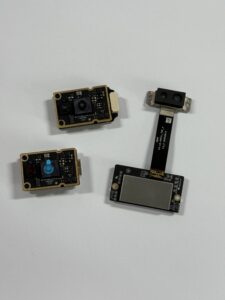
Figure 1: DTOF Solid State LiDAR HM-LD1.
DTOF Solid State LiDAR HM-LD1
The HM-LD1 represents a major milestone in high-performance optical sensing. Solid-state design eliminates the high failure rates associated with traditional mechanical rotation motors, making it highly survivable on high-vibration heavy-duty machines. Its dToF SPAD architecture allows it to confidently operate outdoors. As highlighted in the technical tables, the HM-LD1 maintains sub-centimeter accuracy up to 8.0 meters even under 80,000 lux of direct summer solar interference. This makes it incredibly useful for inspecting civil structures (such as highway bridges, water control dams, and concrete expressways) and deploying unmanned aerial drones for agricultural surveying and powerline corridors, where physical access is dangerous for human technicians.
Optical & Dimensions Datasheet
| Parameter Metric | Specification Details |
|---|---|
| Dimensions (Form Factor) | 43.5mm × 30.0mm × 26.5mm |
| Ranging Capability | Indoor: 0.5m – 25.0m; Outdoor: 0.2m – 8.0m (under 80k Lux) |
| Ranging Accuracy | ±3 cm |
| Field of View (FOV) | 60° (Horizontal) × 45° (Vertical) |
| Weight | 28 grams |
Performance & Hardware Details
| System Parameter | Specification Details |
|---|---|
| Resolution | 40 × 30 (1,200 active pixels) |
| Frame Rate | 10 frames per second (10 fps) |
| Communication Interfaces | UART / UDP / UVC |
| Operating Temperature | -20 °C to 60 °C |
| Power Consumption | 1.2 Watts (5V Input) |
📥 Technical Assets & Documentation Download
To integrate the HM-LD1 solid-state sensor into your current mechanical and electronic platform design, access the official documentation and design brochures below:
Download Link: DTOF SSL HM-LD1 Product Brochure (PDF | 231.81 KB)
For detailed retail information, volume pricing, and immediate evaluation sample supply, visit the official product page:
View Product Details & Pricing ➔
Module 6: Software Integration & Embedded Developers SDK Ecosystem
Hardware capabilities depend significantly on the software supporting them. To streamline integration, the HM-LD1 provides an extensive cross-platform software development kit (SDK) designed for standard industrial computing architectures. You don’t want to spend three weeks writing manual parser registers.
1. Cross-Platform SDK Support
The developer SDK supports three core system architectures:
- ⚙️ x86 Windows (C++ / C# / Python): Designed for rapid prototyping on industrial workstations and simulation testing environments.
- ⚙️ x86 Linux (Ubuntu 20.04 / 22.04 LTS): Tailored for high-end robotic computation hubs and host PCs.
- ⚙️ ARM Linux (Ubuntu / Debian for Raspberry Pi and NVIDIA Jetson modules): High performance with low power draw, ideal for compact warehouse AMRs and light UAV flight stacks.
2. Standard Native Drivers
The HM-LD1 integrates with modern robotic software ecosystems:
- ⚙️ ROS / ROS2 Native Drivers: The SDK includes open-source ROS nodes that output normalized
/point_cloud2and/depth_imagedata streams. This allows system integrators to immediately pipe the sensor’s output directly into standard open-source SLAM algorithms (such as RTAB-Map, Cartographer, or gmapping) and navigation stacks (Nav2) without writing custom low-level device drivers. - ⚙️ UVC Camera Compatibility: Utilizing standard USB Video Class (UVC) drivers, operating systems recognize the HM-LD1 as a standard video source. This simplifies point-cloud processing inside lightweight computer vision pipelines (like OpenCV) and bypasses custom driver installation. This is a massive timesaver on system bring-up day.
Module 7: Developer Knowledge Hub (FAQ)
What is LiDAR, and how does it compare to optical cameras for autonomous mobile robots?
LiDAR (Light Detection and Ranging) is an active sensing technology that calculates absolute physical distance by emitting precise pulses of eye-safe laser light and measuring the Direct Time-of-Flight (dToF) of return echoes. Unlike passive optical cameras, which struggle with depth calculations in low-light, high-glare, or featureless environments, LiDAR sensors produce incredibly accurate 3D point clouds and depth maps in any lighting condition—from pitch-black warehouses to direct sunlight.
Look at the two technologies side-by-side. Passive cameras depend heavily on finding patterns or features in the environment. If you run a camera-based AMR down an unlit warehouse aisle or directly toward a blank white wall, the matching algorithms often fall flat, causing the system to lose localization. LiDAR doesn’t care about colors or patterns. It sends its own physical photons. Also, cameras require massive compute power to perform stereo matching or neural net depth estimation. LiDAR gives you clean, raw spatial vectors straight out of the hardware, which means your single-board computer can focus its processing cycles on navigation and safety code.
For robust, fail-safe AMR navigation, the smart move isn’t to pick just one. Combining active solid-state LiDAR (for highly accurate, low-latency obstacle detection and localized spatial mapping) with optical cameras (for semantic object classification, color-based lane tracking, and deep sign recognition) yields a secure dual-perception setup. This combination ensures reliable operations in demanding, highly dynamic industrial environments.
For industrial robotics and drone development, can I use consumer-grade smartphone LiDAR (e.g., iPhone) as an alternative to industrial sensors?
We get this question all the time in the shop. While consumer-grade smartphone LiDAR is impressive for consumer gadgets, it’s just not meant for industrial robotics, warehouse automation, and drone development. Those consumer-grade designs are optimized for indoor, short-range augmented reality (AR) entertainment, face unlock authentication, and basic 3D scanning. In a real industrial environment, you’re going to hit some hard physical walls.
First off, consumer-grade smartphone LiDAR structures are highly susceptible to outdoor solar noise. Under high-lux sunlight (exceeding 50,000 lux), their detection range drops to less than 2 meters, and depth accuracy goes all over the place. Conversely, industrial-grade sensors like the HM-LD1 utilize high-efficiency SPAD dToF receivers. This allows for stable performance up to 8.0 meters even under direct 80,000 lux solar conditions, making them reliable for outdoor drone altitude-hold and construction surveillance.
Second, smartphone LiDAR operates within closed consumer operating systems (iOS/Android), lacking standard industrial interfaces like UART, UDP, and direct UVC. This makes it challenging to integrate them with common robotic flight controllers, single-board computers, or PLC systems. Industrial sensors are purpose-built to interface directly with platforms like Raspberry Pi, NVIDIA Jetson, or custom flight controllers using lightweight, reliable serial protocols.
Finally, industrial environments subject hardware to continuous mechanical vibrations, shock, and wide temperature swings (from -20℃ to 60℃). Consumer smartphones are not designed for these thermal profiles and lack robust mounting designs, making them highly prone to physical failure in industrial deployments.
Why should robotic developers choose solid-state dToF LiDAR over mechanical rotating LiDARs?
The choice between solid-state and mechanical scanning architectures represents a fundamental trade-off between coverage, physical reliability, and payload weight.
Mechanical rotating LiDARs use internal brushless motors, spinning mirrors, and delicate slip rings to achieve 360-degree horizontal scans. In demanding robotic environments (such as warehouse AGVs traveling over rough concrete or agricultural drones undergoing engine vibration), these moving interfaces are common points of physical failure. Wear and tear gradually reduces measurement accuracy, leading to frequent maintenance and high total cost of ownership (TCO). Solid-state LiDARs like the HM-LD1 containing zero moving parts completely eliminate mechanical wear, yielding long operating lifespans and exceptional MTBF (Mean Time Between Failures).
Additionally, mechanical scanners are bulky, power-hungry (often drawing 5W–15W), and heavy (typically weighing 200g–1000g). This payload penalty drains drone batteries and limits flight times. At just 28 grams with a 1.2W power draw, the HM-LD1 is optimized for lightweight drone gimbals and low-profile robotic sweeps, saving both weight and battery constraints.
Finally, high-impact events—such as hard drone landings, collision bumps, or automated cargo docking—can knock the delicate internal optical paths of mechanical laser turntables out of alignment. Standard solid-state systems integrate the sensor-silicon and emission arrays onto a single monolithic PCB, making them highly resilient to mechanical shock and vibration. This ensures consistent depth sensing in the most demanding industrial environments.
📚 References & Further Reading
- Industry Standard: Learn more about SPAD dToF sensor families on the Sony Image Sensing Division Portal
- Industrial Design: Explore solid-state optical development from the Domi Sensor Technology Resource Hub
- Related Guide: Explore full system specs and documentation on the HM-LD1 Product Specifications Library