How to Choose the Best LiDAR Scanner for Robotics, UAVs, and 3D Sensing: A Complete Developer’s Guide
Choosing the right lidar scanner is one of the most critical hardware decisions for systems architects designing autonomous mobile robots (AMRs), unmanned aerial vehicles (UAVs), and advanced 3D spatial sensing systems. Here is the blunt reality: the market has shifted dramatically from bulky, fragile mechanical spinning assemblies to highly robust, ultra-compact solid-state geometries. This transition has unlocked massive capabilities in embedded perception, but it also demands a deeper understanding of optical physics, data-rate pipeline limitations, and real-world environmental conditions to avoid costly integration bottlenecks. If you make the wrong call here, you will deal with melted batteries, choked CPUs, and robots that go blind the second they step into direct sunlight.
For hardware engineers and software developers alike, selecting a sensor requires balancing optimal spatial resolution, range restrictions, interface protocols, and strict SWaP-C (Size, Weight, Power, and Cost) constraints. This comprehensive guide dissects the underlying tech of solid-state direct Time-of-Flight (dToF) scanning, evaluates critical performance metrics under extreme operating conditions, maps hardware interfaces to embedded operating systems, and details a real-world industrial implementation path. We are going deep into the weeds here, so grab a coffee and let’s get to work.
Table of Contents
- 👉 1. Under the Hood: dToF vs. iToF and the Rise of Solid-State LiDAR
- 👉 2. Critical Parameters for Robotic and UAV System Architects
- 👉 3. Interface Protocols, OS Integration, and ROS Node Configuration
- 👉 4. Deep-Dive Specification Table & Product Hardware Review
- 👉 5. Technical B2B FAQ: Production, Calibration, and Architecture
1. Under the Hood: dToF vs. iToF and the Rise of Solid-State LiDAR
At the core of active optical 3D sensing are two competing methodologies: direct Time-of-Flight (dToF) and indirect Time-of-Flight (iToF). Understanding the physical differences between these methodologies is vital for securing stable ranging over diverse surfaces and under changing environmental conditions. Let’s look at how they actually work under real lab conditions.
Direct Time-of-Flight (dToF) Physics
Direct Time-of-Flight systems measure the actual elapsed travel time of a transmitted light photon. The emitter fires a nanosecond-scale pulse of near-infrared light (often at 905nm or 940nm wavelengths). When the photons hit an obstacle, they scatter, and a portion return to the sensor’s receiver array, which consists of highly sensitive Single-Photon Avalanche Diodes (SPADs).
A high-speed Time-to-Digital Converter (TDC) measures the time delta (Δt) between emission and detection. The distance (d) is determined using the constant speed of light (c):
d = (c × Δt) / 2
Because dToF relies on the arrival of individual photons, it is less susceptible to multi-path interference (where light bounces off multiple walls before returning) and maintains linear accuracy over long distances. This makes it ideal for the open, dynamic environments explored by drones and industrial robots. In the shop, we love dToF because it behaves predictably. Whether your target is 2 meters or 20 meters away, your error margin stays relatively flat. For deeper reading on the optical physics driving SPAD array development, refer to research published by the IEEE Photonics Society.
Another major detail is how dToF handles what we call “photon pile-up.” Since a SPAD operates in Geiger mode, it triggers on the very first photon that hits it. If you have an incredibly bright light source or a highly reflective surface up close, a cheap receiver gets saturated instantly. Premium industrial-grade dToF architectures employ sophisticated active quenching circuits to reset the SPAD in nanoseconds, allowing the sensor to capture subtle returns even from dark, light-absorbing target surfaces immediately after a bright flash.
Indirect Time-of-Flight (iToF) Physics
In contrast, iToF systems emit continuously modulated light (typically sine or square waves) and calculate the phase shift between the emitted and returned signals. While iToF chips can offer higher spatial resolutions at lower price points, they require substantial matching algorithm computations. Additionally, they suffer from phase-wrapping ambiguities at extended ranges and struggle under high ambient light conditions, which can saturate the demodulation pixels and degrade ranging accuracy.
Look at what happens in a tight warehouse corner: an iToF system projects a continuous wave, and that wave bounces off both a nearby concrete pillar and a far metallic rack before returning to the receiver. This causes severe multi-path interference (MPI), confusing the phase calculation and generating a “ghost” artifact in your point cloud. This issue can cause autonomous forklifts to stop suddenly for obstacles that do not actually exist.
The Advantages of Solid-State Architecture
Traditional mechanical lidar scanners use high-speed rotating mirrors, slip rings, and lasers to sweep a 2D or 3D field of view. While effective for highway-speed autonomous vehicles, these moving assemblies are prone to mechanical wear, are sensitive to high vibrations (common on off-road AMRs and multi-rotor drones), and carry high manufacturing costs. If you run a mechanical scanner on a high-vibration engine bay or a quadcopter frame, you can expect the internal optical alignment to drift over time. This means constant recalibration cycles or complete system teardowns.
Solid-state LiDAR (SSL) replaces these moving parts with fixed optical arrays. Operating as flash or addressable matrix arrays, solid-state solutions achieve structural ruggedness, high mean time between failures (MTBF), and low-latency frame rates. This structural durability makes solid-state dToF LiDAR devices an ideal option for physical platforms operating in challenging real-world environments. No motors to fail, no bearings to wear down, and no mirror alignment issues. It is a solid chunk of silicon and optics built to take a beating on the factory floor.
2. Critical Parameters for Robotic and UAV System Architects
Selecting the best lidar scanner requires finding the sweet spot across several key technical boundaries. Evaluating these parameters carefully ensures that your processing pipeline receives reliable spatial data without overloading your onboard compute system. Let’s break down the metrics that actually matter when you are drafting your schematics.
Ranging Accuracy, Resolution, and Field of View (FOV)
The sensor’s spatial resolution determines its ability to resolve fine structural details at a distance. If an AMR must negotiate thin table legs or hanging industrial cables, a single-line scanner can miss the obstacles, while a 3D matrix scanner with an optimized Field of View (FOV)—such as 60° Horizontal x 45° Vertical—will capture them reliably. When you map this layout, you have to look closely at the math behind your coverage area.
Angular Resolution = FOV / Pixel Count
For instance, a 40 x 30 pixel resolution spread across a 60° x 45° FOV yields an angular resolution of 1.5° per pixel. Combined with a ranging precision of ±3cm, systems can detect thin structures, uneven terrain, and sudden drop-offs well within safe deceleration thresholds. This is critical for preventing terminal tip-over events in automated warehouse environments.
Here is the deal with angular resolution: if your robot is moving fast, say 2 meters per second, a wider spot size at a distance means you might miss critical surface details. A target like a 5cm steel pipe hanging in an aisle will only fill a fraction of a wide pixel’s field of view at a range of several meters. The average return signal will make the obstacle look like a minor background variation. Solid-state arrays with distinct, addressable pixels help solve this issue by isolating the target returned energy into dedicated channels.
Ambient Light Robustness and Solar Lux Management
In outdoor environments, ambient sunlight is the leading source of measurement noise. Solar irradiance introduces a high volume of background photons, which can saturate raw SPAD detectors and cause false triggers. To maintain outdoor stability, professional lidar scanners use advanced narrow-band optical bandpass filters and clever signal processing algorithms, such as time-correlated single-photon counting (TCSPC).
Here is how to spot cheap sensors: check their performance curve in high-glare environments. A typical indoor-only sensor will boast a beautiful 20-meter range, but the second you expose it to more than 10,000 lux (cloudy daylight), that range drops off a cliff. When choosing hardware, verify its outdoor range under high illumination levels (e.g., up to 80,000 lux). A sensor that performs well at long range indoors can drop to a fraction of that capability outdoors if it lacks robust solar noise mitigation. Systems targeting dual-mode indoor/outdoor operation must prioritize this high-lux resiliency rating to prevent catastrophic blindness under direct noon sunlight.
SWaP-C Optimization (Size, Weight, Power, and Cost)
For UAVs and battery-powered mobile robots, every gram and milliwatt directly impacts operating time and payload capability. This tri-factor balance determines the overall efficiency of your platform:
- ✅ Mass (Weight): While mechanical scanners can weigh upwards of 500g to 2kg, small-footprint solid-state modules weigh under 30g. Minimizing weight reduces structural inertia, enabling quicker flight adjustments and reducing motor wear on UAVs.
- ✅ Power Dissipation: Many high-performance scanners pull 10W to 30W of power, requiring active cooling systems and draining system batteries. Modern integrated dToF architectures can operate on under 1.5W, simplifying thermal design and extending battery cycles.
- ✅ Integration Volume: A compact housing allows sensors to be embedded flush within robot chassis or camera gimbals, protecting the optics from impact and preserving clean aerodynamic profiles on drones.
3. Interface Protocols, OS Integration, and ROS Node Configuration
Extracting raw depth data and transforming it into actionable spatial coordinates requires a clean hardware interface and a robust software stack. The choice of interface directly affects raw datastream bandwidth, system latency, and CPU overhead. If you’re using a low-power single-board computer (SBC), you have to be highly strategic with how you handle this data pipeline.
Hardware Layer Interfaces: UART vs. UDP vs. UVC
- UART (Universal Asynchronous Receiver-Transmitter): Ideal for resource-constrained microcontrollers (MCUs) like STM32, ESP32, and Pixhawk flight controllers. Serial transmission rates (typically configured at high-speed baud rates like 921,600 bps) stream point clouds containing distance and amplitude data directly into low-level avoidance loops without requiring operating system overhead.
- UDP (User Datagram Protocol): Operates over Ethernet networks, making it the preferred choice for industrial single-board computers (SBCs) like the Raspberry Pi 4/5 or NVIDIA Jetson series. UDP provides low-latency transmission for high-resolution 3D point clouds without the overhead of TCP handshakes, making it highly reliable in multi-device network topologies.
- UVC (USB Video Class): Configures the LiDAR module to register as a standard USB camera. This allows developers to stream depth wraps directly using generic drivers (like OpenCV in Python or C++) without needing proprietary kernel-level drivers. It is the fastest path to proof-of-concept testing on standard PCs.
Operating System Support & Platform Integration
For rapid prototyping and production deployment, search for sensors that offer cross-platform SDKs compiled for multiple architectures. Software development kits must be dynamic, supporting:
- ⚙️ Windows (x86/x64): Mainstream for initial optical testing, calibration, and structural evaluation via graphical user interfaces.
- ⚙️ Linux (x86/x64): Standard for x86-based industrial PCs running Ubuntu or Debian systems.
- ⚙️ ARM Linux (ARMhf/AArch64): Extremely crucial for edge computers like Raspberry Pi and NVIDIA Jetson platforms, allowing local Edge-AI processing, visual slam integration, and real-time path planning.
4. Deep-Dive Specification Table & Product Hardware Review
To ground these performance parameters in a real-world example, let’s explore the physical and electrical specifications of the DTOF Solid state LiDAR HM-LD1. This solid-state module is optimized for low-SWaP-C applications, offering robust, long-range 3D perception in an ultra-compact package. Let’s look at how the physical integration values map out.
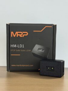
Figure 1: Product and outer packaging
Master Specifications: DTOF Solid-State LiDAR HM-LD1
Below is a detailed breakdown of the module’s key dimensional, optical, and operational standards. For complete system schematic diagrams and mounting patterns, you can download the official DTOF SSL HM-LD1 Product Brochure.
Performance Analysis & Implementation Strengths
The hardware architecture of the HM-LD1 makes it uniquely suited for space-constrained and weight-sensitive applications. If you’re building a drone or a compact AMR, here’s what this hardware gives you under actual field conditions:
- ✅ High-Lux Outdoor Performance: A common point of failure for lightweight LiDARs is outdoor operation under direct sunlight. The HM-LD1 maintains a robust range of up to 8 meters even under intense 80,000 lux solar loads—comparable to bright, direct summer sunlight. This outdoor capability makes it highly dependable for UAV terrain-following, obstacle avoidance, bridge inspections, and industrial crop surveying.
- ✅ Compact, Low-Mass Envelope: Weighing just 28 grams, this module is light enough for micro-UAVs (under 250g takeoff weight) and small AGVs, serving as a primary sensor for collision avoidance and altitude hold without dragging down battery life or dynamic flight capability.
- ✅ Low Power Requirement: Consuming only 1.2W, the sensor generates very little heat. This allows engineers to enclose it in sealed, dusty, or wet housings without needing heavy heatsinks or cooling fans.
- ✅ Highly Compatible: Built-in SDKs support development across Windows, x86 Linux, and ARM Linux, making it easy to integrate with PCs, Raspberry Pi modules, and microcontrollers.
View Product Details & Pricing ➔
5. Technical B2B FAQ: Production, Calibration, and Architecture
Q1: Is an iPhone LiDAR scanner sufficient for professional B2B applications, VFX, or robot navigation?
Consumer-targeted smart devices operate on low-power, non-adjustable eye-safe VCSEL emitters paired with wide-field optics. The primary limitation of consumer setups becomes clear under bright sunlight: on-chip filtering is optimized for indoor comfort, and direct outdoor sunlight can easily overwhelm the sensor, reducing its effective range to less than 1.5–2 meters. Additionally, consumer operating systems (like iOS) restrict developers behind a closed SDK. This limits raw depth access, adds processing latency, and prevents direct serial hardware handshakes.
Furthermore, integrating an iPhone into an active robotic platform introduces mechanical and logical integration challenges. It lacks typical industrial physical interfaces (such as standard UART, UDP, or USB-UVC), does not support direct mounting points, is sensitive to vibration-induced battery disconnection, and cannot communicate directly with real-time Robot Operating System (ROS) nodes.
For professional tasks that demand direct execution, real-time 3D point clouds, stability under high outdoor solar loads (up to 80,000 lux), and flexible interfacing, a dedicated industrial solid-state dToF module like the HM-LD1 is the superior choice. If you try to mount an iOS device onto an industrial AMR, you are asking for a maintenance nightmare.
Q2: Can I integrate these LiDAR scanners into DIY projects or low-cost Raspberry Pi platforms?
When integrating with a Raspberry Pi, keep the following hardware considerations in mind:
1. Power Configuration: The HM-LD1 draws a modest 1.2 W at active load (about 240 mA at 5V). This is easily handled by the Raspberry Pi’s onboard 5V GPIO headers or a standard USB port, eliminating the need for complex, heavy step-down voltage regulators.
2. Interface Driver Choice: You can connect the sensor using the onboard UART pins (/dev/ttyAMA0 or /dev/ttyS0), stream data over a local Ethernet connection via UDP, or register it as a plug-and-play UVC camera over USB.
3. Software Setup: Hardware kits typically include pre-built C++ and Python SDK libraries packaged for ARM-based Linux distributions. This allows developers to read the 40×30 depth array, apply software filters, and convert the raw distances into real-time PointCloud2 maps in minutes, without writing low-level drivers from scratch.
Q3: What parameters waste budget if they aren’t optimized for UAV or robotic navigation?
1. Mounting High-Power, Long-Range Scanners on Short-Range Systems: Purchasing a 150-meter range scanner for an indoor autonomous mobile robot (AMR) or a drone that flies primarily at 5-meter altitudes is a wasted expense. High-range scanners (which typically rely on high-power Class 1 infra-red lasers) are significantly more expensive and carry strict power demands, often requiring 15 W to 30 W of power. This high draw generates considerable heat, requiring heavy active heatsinks or cooling fans that add bulk and reduce reliability.
2. Overlooking Sensor Weight on Flying Platforms: For unmanned aerial vehicles (UAVs), every gram of payload weight cuts into operational flight time. Opting for a heavy, mechanical spinning scanner (often weighing 300g to 800g) when a lightweight 28-gram solid-state dToF sensor can handle close-range obstacle avoidance and altitude hold can significantly impact performance. By matching your range requirements directly to the flight envelope, you can save system weight and allocate that capacity to carrying larger batteries or specialized camera gear.
3. Neglecting Outdoor Ambience Ratings: On the flip side, some system architects try to save money by choosing inexpensive, indoor-only phase-shift iToF depth cameras, only to see performance drop to near-zero under the glare of outdoor sunlight. If your robot or drone needs to transition between indoor warehouses and outdoor loading zones, choosing a sensor with built-in solar noise suppression (capable of handling up to 80,000 lux) is a critical requirement. This ensures consistent performance in changing conditions, saving you from costly redesigns down the line.
📚 References & Further Reading
- Industry Standard: Reference benchmarks on professional solid-state sensor array packages can be reviewed through Sony’s Depth Sensing Solutions.
- Standard Bodies: For comprehensive research on active optical SPAD array architecture, explore the IEEE Photonics Society publications.
- Related Product Guide: Read specifications and integrate micro-sized dToF modules by exploring the DTOF Solid State LiDAR HM-LD1 product page.